What is a Shuffle Box?
Understanding the passive optical technology that eliminates the core tier in 100,000+ GPU AI clusters and why it's becoming essential infrastructure knowledge.
Stephen Klenert
SVP, Optical Network Operations · 365 Data Centers
I've been building and running fiber networks for a long time. And right now there's a concept spreading through AI infrastructure design that most people in the industry either haven't encountered yet or are getting wrong. I got it wrong myself the first time someone asked me about it.
It's called an optical shuffle. It sounds simple. It isn't — or rather, the concept is simple but the implications are significant enough that if you're building or operating AI cluster infrastructure and you don't understand it, you're going to make expensive mistakes.
What a shuffle actually is
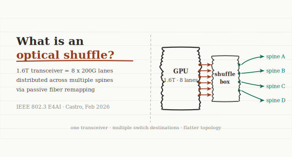
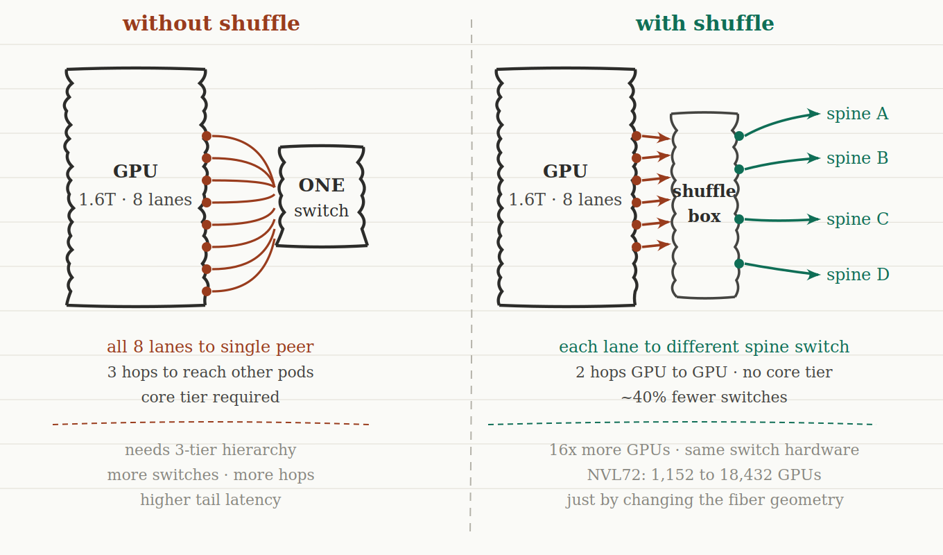
Start with a modern high-speed transceiver. A 1.6T DR8 runs 8 parallel optical lanes at 200G each. In a conventional network connection, all 8 of those lanes terminate at a single switch port on the other end. One transceiver, one peer, one connection.
An optical shuffle breaks that assumption. It takes those 8 lanes and physically remaps them — distributes them — to different switch ports, potentially on completely different switches. Lane 1 goes to Spine A. Lanes 2 and 3 go to Spine B. Lanes 4 and 5 go to Spine C. And so on. The GPU node still has one transceiver. But now it has direct optical connectivity to multiple independent spine switches simultaneously.
The device doing that remapping is the shuffle box — a passive optical module, no power, no active electronics, no management interface. Just precision fiber geometry that routes each incoming lane to a different physical destination.
This is fundamentally different from a breakout panel or an MPO cassette. A breakout exposes individual fibers 1:1 from a multi-fiber connector — the positions don't change, fiber 1 in is fiber 1 out. A shuffle deliberately reorders and redistributes the lane assignments to achieve a specific topological outcome. The remapping is the product.
The shuffle eliminates the core tier — passive fiber geometry does the work of a whole switch layer.
Why this exists — the topology problem it solves
To understand why shuffles matter, you have to understand the problem they're solving in large AI clusters.
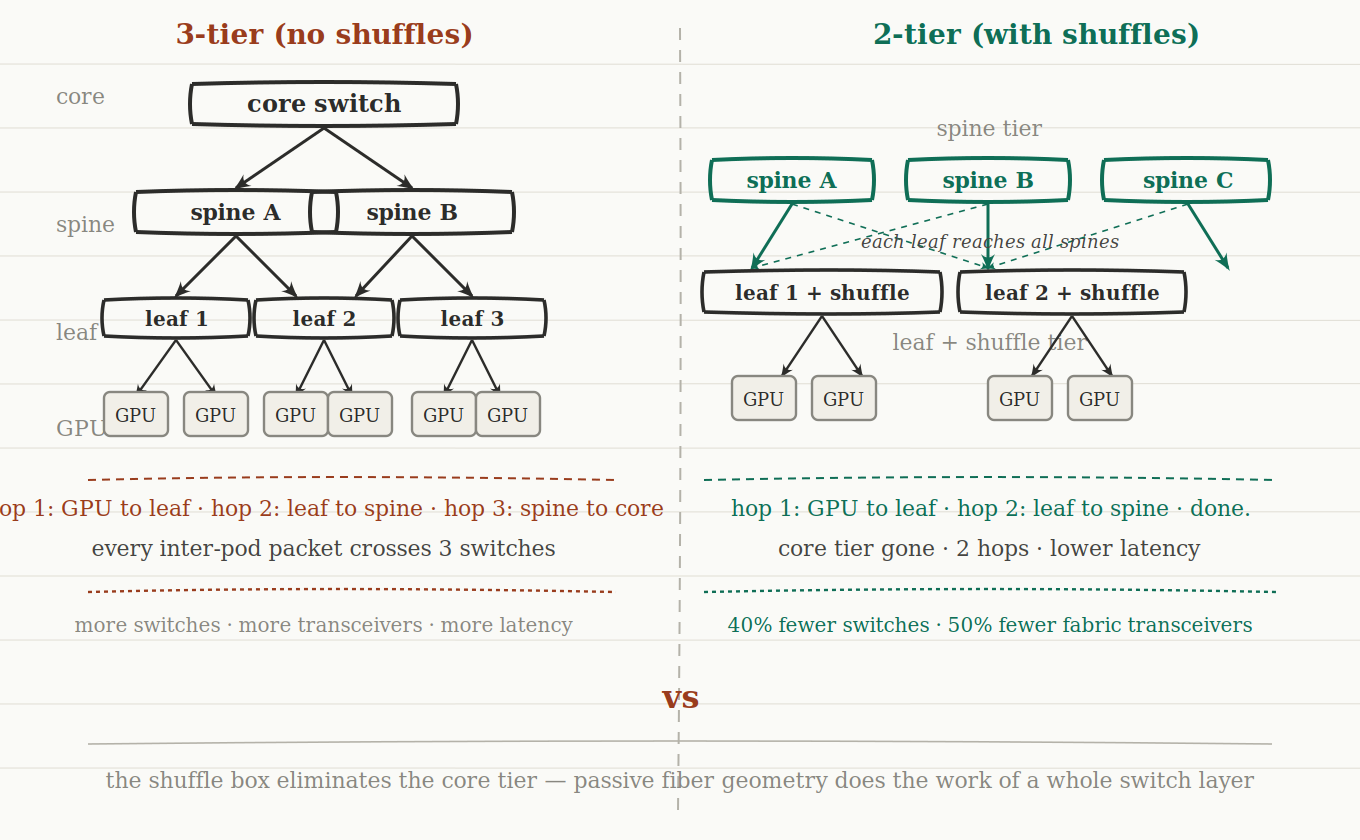
A traditional 3-tier leaf-spine-core network works fine for general data center traffic. Packets hop from server to leaf, leaf to spine, spine to core, then back down. Three switching hops between any two servers in different pods. The core tier exists because without it, every leaf switch would need a direct link to every other leaf switch to maintain full any-to-any connectivity — which doesn't scale.
In AI training workloads, those extra hops have a real cost. GPU collective operations — all-reduce, all-to-all, broadcast — are latency-sensitive. The network is on the critical path of every training iteration. Each additional switch hop adds switching latency, queuing delay, and another potential failure point. At 100,000-GPU scale, the aggregate effect is measurable in training throughput.
The optical shuffle is what makes it possible to eliminate the core tier entirely.
How the shuffle enables 2-tier fabric
When each GPU node's transceiver lanes are distributed across multiple spine switches via a shuffle, each node has direct optical reach to a wide slice of the spine layer in a single hop. Leaf switches can now connect directly to all spine switches because the GPU's own transceiver — through the shuffle — is already spreading load across them.
The core tier's job was to aggregate connectivity between spines. The shuffle does that at the physics layer, for free, without an extra box.
The result is a 2-tier fabric — leaf and spine, nothing above. From the February 2026 IEEE 802.3 E4AI presentation by Jose Castro at Corning: roughly 40% fewer switches, 50% fewer fabric transceivers, and about 33% total transceiver reduction including GPU-to-leaf links. Two fewer switch hops per flow. Meaningfully lower tail latency.
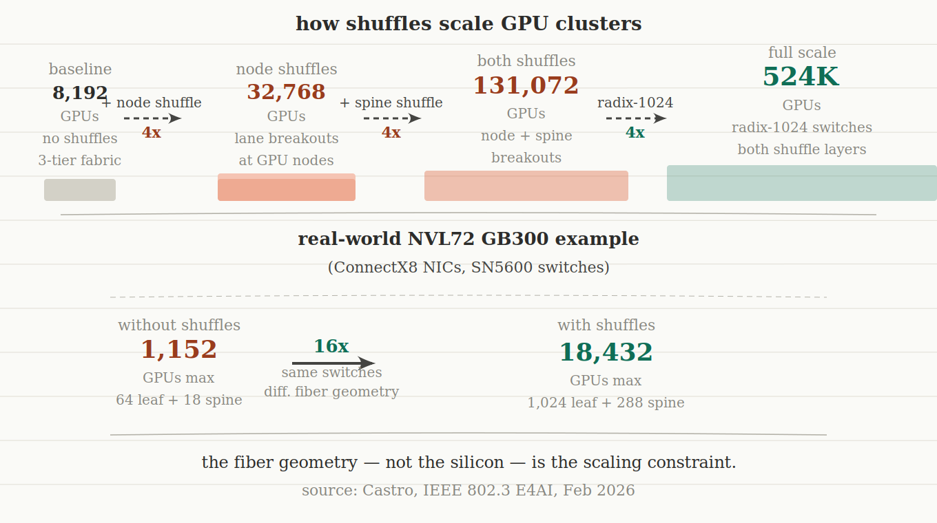
Without shuffles, the NVL72 GB300 cluster with ConnectX8 NICs tops out at 1,152 GPUs. Add shuffles — same hardware — and you scale to 18,432 GPUs. That's 16x growth just from changing the fiber geometry.
What the numbers look like
Take a cluster built around NVL72 GB300 nodes with ConnectX8 NICs and SN5600 switches. Without optical shuffles, using a conventional topology, the maximum cluster size you can build tops out at around 1,152 GPUs — 64 leaf switches and 18 spine switches. That's the ceiling imposed by the topology, not the hardware.
Add optical shuffles. Same switches. Same NICs. The ceiling moves to 18,432 GPUs — 1,024 leaf switches and 288 spine switches. That's a 16x increase in addressable cluster size driven entirely by changing the fiber geometry, not by upgrading any active hardware.
Push further with higher-radix switches and shuffle layers at both the node-to-leaf and leaf-to-spine levels, and the IEEE analysis shows paths to 131,000 GPUs on a 2-tier fabric, and 524,000 GPUs with radix-1024 switches. At that scale you're talking about 524,000 duplex fiber connections per fabric plane.
That last number is the one that should stop you cold if you're thinking about operational implications.
The three implementation forms
The IEEE paper describes three ways to physically implement optical shuffles, and they have real tradeoffs worth understanding before you specify anything.
Integrate the lane remapping directly into the cable assembly. The cable legs are staggered at the factory so different fibers land on different switches right out of the box. No separate module, minimal rack space. The tradeoff: troubleshooting — when something goes wrong with a harness, isolating the problem fiber is harder than with a modular approach, and you can't swap individual components.
The modular option. Small form factor, easy to replace as individual units, straightforward to document per-port. Good for smaller deployments and situations where flexibility matters. The downside: rack space efficiency — at very large scale, the cumulative footprint adds up.
The high-density choice. Higher port count per rack unit than cassettes, designed for the scale of interconnect that 32,000 or 131,000 GPU clusters require, relatively easy to replace as a unit if damaged. This is the form factor showing up in the largest AI builds being designed right now.
There's also emerging photonic technology worth knowing about — 3D waveguides written directly into glass using laser fabrication. These minimize crossovers and crosstalk compared to planar optical flex circuits. It's not commodity product yet, but it's a real direction and it's moving faster than most people expect.
The device is completely passive. No management interface. No link state. No alarms. If a fiber is in the wrong port, nothing in the hardware tells you.
The operational weight
Here's what I think doesn't get enough attention in conversations about optical shuffles: the device is completely passive. No management interface. No link state. No alarms. If a fiber is in the wrong port of a shuffle module, nothing in the hardware tells you. The network might still come up — with a degraded, asymmetric path that quietly tanks your training throughput while you spend hours looking at switch logs.
At 131,000 GPU scale, the paper notes that manual lane shuffling during deployment is simply not feasible. The connection count is too high. And next-generation transceivers will add optical link training requirements that further constrain which lanes can legally connect to which ports — meaning the shuffle configuration can't be arbitrary. It has to be engineered before deployment and documented precisely.
The shuffle configuration — which GPU lane maps to which spine switch, through which shuffle module, at which port position — has to exist in your cable schedule before a single fiber is pulled. Not discovered during commissioning. Not reconstructed after the fact from photos. Designed, documented, and verified.
In a fat-tree AI cluster built for packet spraying, path diversity is a design assumption baked into the routing layer. If your physical fiber geometry doesn't deliver the path diversity the routing table expects, your traffic engineering breaks silently. You don't get an error. You get slower training and a debugging session that points everywhere except at the shuffle module where the problem actually lives.
What this means for the industry right now
If you're designing an AI cluster — at any scale where you're building your own fabric — the question isn't whether optical shuffles are relevant. They are. The question is which implementation form fits your scale and operational model, how you're going to engineer the lane assignments, and how you're going to document and maintain the physical layer going forward.
For colocation and data center operators: your customers building large GPU clusters are going to ask about shuffle-aware structured cabling infrastructure. The customers designing 10,000+ GPU builds are already past the point where conventional patch panel topology works. This is not a future consideration. It's in active RFPs right now.
The optical shuffle is one of those Layer 1 concepts that sits quietly under everything else — under the routing, the fabric software, the GPU drivers, the ML framework — and either enables the performance the system was designed for or silently constrains it.
Understanding it isn't optional for anyone building serious AI infrastructure in 2026.
Technical reference: Castro, J.M., “Optical Shuffle Architectures for Large AI Networks,” IEEE 802.3 Ethernet for AI Assessment Ad Hoc, February 2026.
Save this article for later
Download as PDF to read offline or share